Tag: 18th Century

  • The Death of a New World: Disease and Population Decline In South America from 1492 to 1800CE

    Preface: A Subject of Scale

    In its whole, the story of population in South America from 1492 to 1800CE is one of demographic collapse. At the low point of this period the continent would be witness to a population that reached but 1/5th the size of its pre-Columbian standard. However, taken individually, the huge variance in experience within South America during this period becomes apparent; from regions whose population figures fall and rise in dramatic peaks, to those that undulate composedly across modest crests.

    Initially however, it is important to note the vast scale of this undertaking and the limitations therefore imposed, namely a limitation to the macro. Many of the studies concentrating on South-America in this field have been of a type that focus acutely on one specific area and are successful in realising the demography of such a space in fine detail. These studies range in size from David Noble Cook’s study into Peru over a period of 100 years to Brian M. Evans’ study of an Andean Village over a period of 43 years. The view herein over all South America over 308 years will draw on studies such as these but will not attempt to replicate them in outcome. The expansive scope of this article requires it to correlate broader trends and seek to contextualise them within a continent-wide context. This is a complimentary approach to the mathematical facet of this study which operates more effectively with larger pools of data. The ultimate achievement of this article is to plot the change of the indigenous and total population of South America over this period, as a collation of other studies done in this area alongside primary census data. Moreover, it will explain to what extent disease was the primary causation for demographic change and shall provide offerings as to the variance in population decline across five distinct regions within South America (see figure 1.). Furthermore, when the term ‘disease’ is used herein it is used as a collective term for multiple afflictions; this is due to the fact that there is much dispute as to which diseases affected which populations at what times, although it is generally accepted that smallpox, measles, and typhus were the main killers with the Variola Major strand of smallpox constituting the greatest killer overall.

    The standard disclaimer must be applied here that the figures presented herein, although primarily drawn from census data of the period and believed by the author to be broadly correct, are bound inevitably to be inaccurate in many aspects. This is the challenge of applying a scientific approach to historical data. However, dealing with incomplete source material is the perpetual challenge of the historian and one that cannot be shied away from, lest no history be written at all.

    Pre-Columbian South America

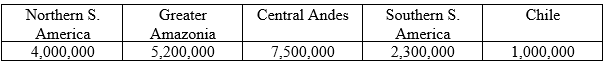
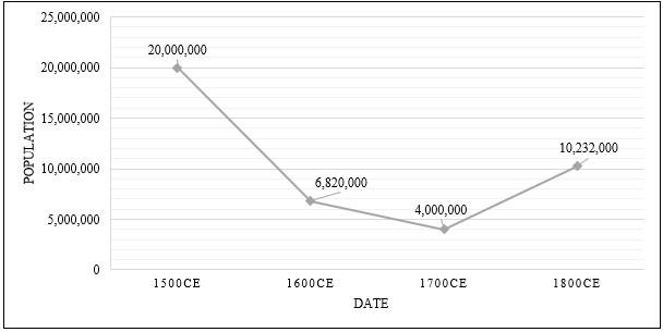
    Before we begin to assess change across the continent we must first be clear in what we are assessing a change from. What was the makeup of South America in 1492?  Estimates for the overall population for the region continue to exist in dispute however some mean figures have been produced for this article, in aggregation of several other estimates made over recent years. The central influence for these pre-Columbian figures continues to be the work of William M. Denevan and his text The Native Population of the Americas in 1492 which remains an excellent source on this topic. Ultimately the total population statistic reached for pre-Columbian South America in 1492 is 20,000,000. Across this study, this total figure is broken down into five regions across South America. These are: Northern S. America, Greater Amazonia, Central Andes, Southern S. America, and Chile. The continent has been split this way partially due to geographical differences in the five regions and partially to facilitate cross-comparison over time. If we were to use boundaries that shifted over time, such as the borders of nations, our comparisons would be less accurate. These borders are approximates of regions and are not intended, nor should not be taken, as accurate boundaries.

    Figure 1. Map of Identified Regions of South America

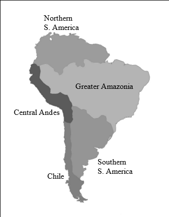
    The regions identified in figure 1 are the geography to which the rest of this article is referenced to. Thus, the population split for South America in 1492 is as presented below.

    Figure 2. Table of Pre-Columbian Populations in South American Regions

    These demographics aside, what other features can we ascribe to these five regions that might be important in a study of post-Columbian disease spread? For this study the focus lies on significant factors that can be compared across the five regions identified. These are: climate, geography, and patterns of settlement.

    In terms of climate, for which the Köppen-Geiger climate classification system is used, our two most northerly regions of Northern S. America and Greater Amazonia can be described as ranging between a tropical (Aw) and equatorial climate (Af). These warm and wet conditions which comprise the great majority of these two regions are well suited to the spread of disease, particularly as they are prone to monsoon; we would therefore expect higher levels of mortality in these regions than in others. The Central Andes region contains a greater variance in climates due to its mountainous geography: it is mostly covered by a cold desert climate (BWk) but also contains large areas of semi-arid climate (BSk) and temperate oceanic climate (Cfb). We would expect these colder and drier conditions to be more effective at staying disease spread here. The Southern S. America region would mostly be classified as a warm oceanic climate (Cfa) with some areas of tropical (Aw) and semi-arid climates (BSh). This region can be described as susceptible to the spread of disease but not to the extent of Northern S. America and Greater Amazonia. Finally, in Chile we find areas of cold desert climate (BWk), temperate Mediterranean climate (Csb), and temperate oceanic climate (Cfb). This, in similar fashion to the Central Andes, is an area we would expect to find reduced mortality rates in due to these pathogen-hostile climatic factors.

    The geography of the continent can be split into two areas on either side of the Andean mountain range which covers the regions of the Central Andes and Chile. These mountains are a dominant factor in the lower temperatures seen in these regions as discussed above. Additionally, the mountains help to curtail the spread of disease by limiting travel and isolating groups from one another. On the eastern side of this “Andean split” in Northern S. America we can identify the Guiana highlands as a geographical feature that would act similarly. This is also true for the Brazilian highlands in Greater Amazonia and Southern S. America. However, these highland areas will prove less effective at preventing disease spread in these regions as they do not cover them in entirety, unlike with the Andes, and thus their major comprisal of large lowland areas still allows disease to spread more efficiently.

    For patterns of settlement across the continent: in clear majority we are discussing a dispersed population of peoples that do not gather into large permanent communities. This is the case for Northern S. America, Greater Amazonia, Southern S. America, and Chile. Certainly, there were areas of more concentrated populations within these regions, often along rivers and coastlines, but these were still clusters of villages rather than towns or cities. This type of isolated pattern of settlement is one which is often effective in curtailing the spread of disease, so we would expect regions with this pattern to be less susceptible to illness. In 1492 the exception to this rule was the area of the Central Andes, occupied in majority by the Inca Empire which was home to cities with populations of 700,000 or more such as Cusco, Quito, and Choquequiaro. In this case we would expect to see this area prove more susceptible to disease spread than others.

    Three Hundred Years of Disease in South America

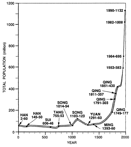
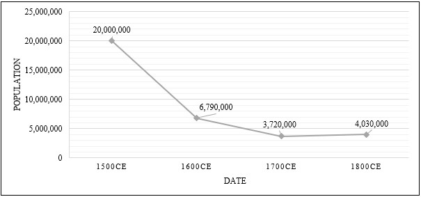
    Population figures across this period, particularly during the first 100 years, are to be taken with a large margin of error. After 1600 the Spanish and Portuguese began taking censuses of the regions they controlled, spanning by this point almost all the continent, and so we do have primary statistics available to us that were not available for our pre-Columbian assessment. Even so, it is highly likely the numbers they give are low estimates, as even today our estimates ever increase for the number of indigenous on the continent. Nonetheless, by collating all these censuses in conjunction with our pre-Columbian estimate we can produce a graph that tracks the population of the continent over these 300 years.

    Figure 3. Graph Plotting the Population of South America from 1500 to 1800CE

    Using this data, we can also calculate the rate at which the population changes between these points, as seen in the table beneath.

    Figure 4. Table of Total Population Rise and Fall (%) in South America 1500-1800CE

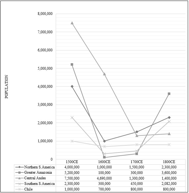
    These statistics show the immediate damage done to the continent and the recovery from that. However, it must be noted that these population statistics are not solely for indigenous peoples, they include all those people who have, either by choice or by force, moved to the continent during this time. This is what explains the 155.8% increase in population from 1700 to 1800, it is comprised of immigration, we would not expect a native population to recover at this rate. The question therefore asked becomes what is the rate of native population recovery, as supposed to simple population increase overall? For this we can utilise our regions; by splitting our demographics between these five zones, including those that saw large immigration and those that didn’t, we can determine the extent to which immigration as a factor has affected the overall population statistics. 

    Figure 5. Graph Plotting the Population of Regions of South America 1500-1800CE

    For this above graph we can also produce a population change rate table.

    Figure 6. Table of Population Rise and Fall (%) in Regions of South America 1500-1800CE

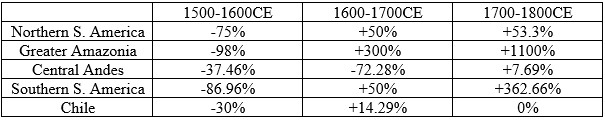
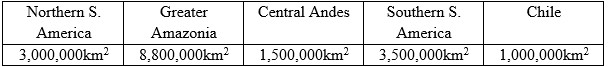
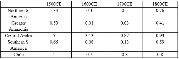
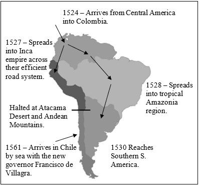
    This information is enlightening in multiple aspects. From 1500 to 1600 we can immediately see that some areas have declined to far greater extent that others, namely Northern S. America, Greater Amazonia, and Southern S. America have declined at much higher rates that Chile and the Central Andes. This can be explained by the climates and geography of these regions which, as was explained above, are far more suited to preventing the spread of disease in the Central Andes and Chile than in the other regions. In Chile this can be further explained by noting that disease did not reach the region before 1561, much later than the other regions (see figure 9.). However, some Umbridge must be taken with the 98% decline figure for Greater Amazonia during this period. Of all the data drawn on for this study this figure seems the most inaccurate. Although it may well be true that mortality rates were high in this region due to its tropical climate, the 0.59 population density for this area would never allow such a drastic reduction (see figure 8.). This article would hazard that the rate of reduction would be closer to the 75% reduction seen in Northern S. America as these two regions have very similar climates and geographies. Nevertheless, in the absence of any further data the -98% figure will continue to be used.

    From 1600-1700 the notable standout is the one region which continues to decline whilst the others begin to rise in population, the Central Andes. This is likely explained by the concentrated population density in this region which allowed for disease to continue to spread virulently, as seen in figure 8. By 1600 the other four regions all have populations densities beneath 1 compared to the Central Andes which sits at 3.13. At this point it may well be argued that these other four regions have reached a point beneath the ‘minimum concentration of hosts’ threshold whereas the Central Andes has not; this means their populations are now too small when compared to the size of their landmass to facilitate further disease spread. The well-developed road system of the Incas will have also allowed continual consistent movement of peoples around the empire; further facilitating dissemination of infection. This is especially crucial if you note the long incubation period of the two largest killers, smallpox and measles, which exist in the body for c.10 days before the person infected begins to show symptoms. The further a person is enabled to travel within these 10 days the faster these illnesses can spread. We can also see within the regions whose populations do rise the difference in the rates of the population increase. This is explained by immigration, not native recovery, and will be explored in depth with the assessment of the data between 1700 and 1800.

    Figure 7. Table of Landmass Area of Regions (km2)
    Figure 8. Table of Population Density of Regions Within South America (Number of Persons Per km2) from 1500-1800CE

    From 1700-1800 we can clearly identify the regions which are experiencing outside immigration and those which are not. Again, we see a divide made between the Andean regions of Chile and the Central Andes and the rest of the country. On the west side of the Andean split we see population figures that are struggling to begin a recovery towards pre-Colombian levels, with Chile’s population becoming stagnant and seeing no increase in the 100 years between 1700 and 1800. This is representative of how the native population across the country is recovering from the impact of disease: slowly. The reasons for this are numerous; one large factor is a decrease in fertility rates after disease has ravaged a population. This can be due to the disease itself physically affecting reproductive abilities or unbalancing the gender ratios in a population but can also be a result of social grief and stress. Recovery rates are also affected in the long term because disease results in higher mortality rates in the young population, who are the ones able to reproduce.

    Figure 9. Map Depicting the Spread of Disease Across South America 1524-1561CE

    With our knowledge of the western side of the Andean split the extraordinary nature of the figures from the eastern side becomes apparent. Even the 53.3% increase seen in Northern S. America would be classed as an unprecedented event, with figures of over a 1000% increase existing in realms of fantasy. These statistics correlate well with the records kept by the Spanish and Portuguese of slaves imported during this period, which indicate c. 5,000,000 were imported into the Viceroyalties of Brazil, Rio de la Plata, and New Granada from 1700-1800. Using this data we can calculate how much of the increase in population on the east side of the Andean split is due to immigration. Taking Greater Amazonia as our example, given that it saw the greatest increase in immigration, we can take 10% as a generous figure for the increase in native population during this period. This would constitute only 30,000 of the 3,300,000-increase seen in population and means that 99.16% of the new population is imported. Using similar thought we can interpolate new data across all our existing figures produce a graph that tracks only the indigenous population statistics

    Figure 10. Graph Plottingthe Indigenous Population of South America 1500-1800CE
    Figure 11. Table ofIndigenous Population Rise and Fall (%) in South America 1500-1800CE

    Now we have calculated the decrease in native population we must ask: to what extent is disease responsible for these deaths? It is understood that it is the major factor, but how far so? Let us examine the Spanish and Portuguese maltreatment of the indigenous to see the extent of their impact.

    Figure 12. Table of Conflicts Within South America 1492-1800CE

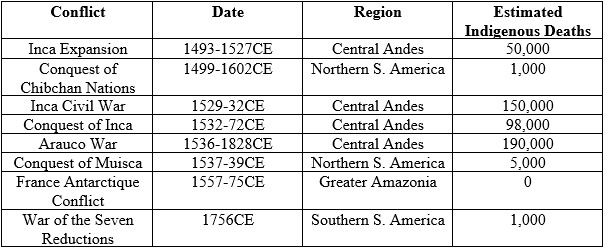
    It is evident from this information that death from conflict may be considered a negligible factor when considering the overall indigenous population decline of South America. The single conflict with most meaningful impact on population is the Inca civil war which accounts for only 1.1% of the population decline from 1500 to 1600. The Arauco war is the cause of the most deaths but stretched over a far longer period, giving it less impact.

    As for the encomienda and mita systems, alongside other forms of cruelties brought about by the Europeans, it is unknown how many died as a direct result of these persecutions as no records were kept, not even estimates. These, evidently, were not numbers the colonisers wanted recorded. Even if we did have such data it would be difficult to extricate deaths directly caused via cruelty and those that came tangentially because of it. We may still make some assessment of their material impact however; the one undisputable fact is that these systems helped facilitate the spread of disease through multiple means. They gathered previously dispersed populations into concentrated groups, forced them to travel long distances, and worked them into a state of weakness. All of which are ample conditions to facilitate infection. In this sense their impact on population decline may have been far greater than they are given credit for here. Nonetheless the ultimate cause of death is disease in majority by a far margin, as far as our statistics show us.

    If we take our statistics from figures 10 and 11 and subtract population decline for reasons aside from disease we can produce an estimate of indigenous population decline specifically as a result of disease. We have calculated that approximately 1% of the population die as a result of warfare between our 100-year intervals, using a global average we can also calculate that approximately 1% can be accounted for by “natural causes” and accident. As discussed there are no statistics for the impact of systems such the encomienda but we must estimate they had some impact given the severity of their programmes, and have been given a 2% impact factor. Overall these account for 4% of the total indigenous population decline from 1500 to 1800. The total indigenous population decline from 1500 to 1700 (it’s lowest point) is 81.4%, so therefore the total decline as a result of disease before the population begins to rise is 77.4%. This means the total number of indigenous killed by disease from 1500 to 1700 is 15,480,000. It must also be noted for clarity that even after this point, as the population increases, indigenous peoples are still dying from disease and that some of these infections continue to plague areas of South America in the 21st century. 

    Ultimately this article has been able to track the population, indigenous and otherwise, of the South American continent from 1492 to 1800. It has provided reasoning for the variance in figures seen across the five identified regions and compared them against each other to infer further detail about the impacts of disease and other factors during this time. Although it is understood that these figures are approximates, it is nonetheless understood their significance in helping us understand this troubled period of history.

    Author/Publisher: Louis Lorenzo      

    First Published: 19th of October 2018

    Last Modified: 23rd October 2018 (Clarity)

  • Piracy and Social Banditry

    For as long as there has been sea-faring trade, there have been people who seek to exploit its riches; pirates, the ‘enemies of all mankind’. To describe pirates, a group traditionally known as quintessentially villainous, as “social bandits” seems initially preposterous but the more we learn about their egalitarian societies the more plausible this description becomes. For this article I am using Eric Hobsbawm’s definition of social banditry, namely:

    ‘peasant outlaws whom the lord and state regard as criminals, but who remain within peasant society, and are considered by their people as heroes’

    In this article I will be considering various aspects of piratical society and whether these aspects allow the pirate to fall into the category of “social bandit” described above or otherwise. Assessing whether pirates match the four main requirements stipulated above of being ‘peasant’, ‘criminals’, ‘within peasant society’, and ‘considered by their people as heroes’.

    Firstly, can pirates be described as ‘peasant’? The answer to this is comprehensively that they can. Although there were some notable exceptions, such as with the case of Major Bonnet, the average pirate was both poor and of low social status, the very quintessence of peasant-hood. Marcus Rediker describes pirates as ‘dispossessed proletarians’, people who saw piracy as a chance to increase both their social and monetary wealth. As well as this piracy also represented a form of counterculture, a certain freedom and liberty outside of the existing social order. Many similarities can be drawn between becoming a pirate and moving to stay in the colonies, Paul Gilje explains that in both cases individuals were given ‘the chance to make many decisions of their own accord’. This ideal of rebellion against society is one central to the notion of the social bandit because it insights antagonism against the ruling elite and association with the “common people”. Pirates would generally have already held a maritime occupation of low social standing before their stint as outlaws; they may well have been fishermen, crews on merchant vessels, or privateers. As such, the difference in lifestyle between the two roles was often not very different and made it easy for those of pre-existing peasant status to convert to piracy. For those of high social status it would constitute a particularly exhaustive change in lifestyle to become a pirate and this is one prominent factor in deterring such classes.

    Secondly, were they regarded as ‘criminals’ by officials and the state? This is also a definite positive. Pirates were agreed to be criminals not only domestically, but also on the international stage as they attacked all factions active in the Atlantic including the British, French, Dutch, and Spanish. This is because, as Kris Lane identifies, pirates did not pose against any individual nation, but against the very ideal of nationhood itself through an ‘almost universal rejection of national and religious authorities’. As Amedeo Policante states, piracy created the need for an international legal response, the Ius Publicum Europaeum (“European Public Law”). This meant the removal of amity lines between European states and the ‘collective appropriation of the oceans’. Phil Steinberg argues that with this framework in place any ship not attached to a nationality could thence be apprehended as an agent of the ‘anti-civilisation of the sea’. A 1696 case against Captain Avery’s crew led an English judge to rule that he had ‘jurisdiction over all people – anywhere on earth – who interfered with English commerce’, this was a direct criminalisation of piracy. Charles Johnson’s 1724 text on piracy shows us that pirates were actively punished and that the laws set against them were used in practice, not only in theory. He vividly describes the numerous public executions of the pirates he describes within his text and how their deaths were to be “without Benefit of Clergy, and forfeit Land and Goods.” This form of dishonourable execution is evidence of the authorities’ specific disdain for criminal piracy.

    Thirdly, did pirates ‘remain within peasant society’? In other words, did piracy remove people from their “roots” or did pirates continue to care about the welfare of those still within the peasant society they left behind? This question is less clear-cut to answer as the previous two but on balance I do believe that this is also the case. Certainly, there was a universal community between pirates themselves, who were willing to cooperate with each other ‘even when the various crews were strangers to each other’. Indeed, in many ways pirates led more inclusive societies than their landlubbing adversaries; according to Richard Burg they promoted a ‘multicultural, multiracial, and multinational social order’. This meant pirates were able to not only remain within peasant society, but expand it to include people of varying backgrounds. Also, since it was highly unlikely any individual pirate would survive more than three years a-sea there was a constant influx of new peasants joining pirate crews and these kept pirates close to the peasant societies from which they came. However, this does not detract from the fact that pirates, in the end, held allegiance only to themselves and would not shy away from putting any peasant to the cutlass should they refuse to join their crew. This is likely why so many captured seamen “volunteered” to join pirate crews, which was favoured because it was thought this would create a better social cohesion between the sailors. Female pirates were also expressly banned on pirate vessels by the pirate code. This does not show express antagonism towards peasants however, because pirates were indiscriminatory in this sense, and would give the same treatment to any person who would defy them. Pirates were also far more inclusionary toward people with disabilities, which would be disproportionately those of the peasant classes; it is not coincidence the peg-leg and the eye-patch are engrained onto the modern perception of the pirate. Indeed, pirates were the authors of the worlds first workers compensation scheme whereby sailors could be paid for their injuries sustained. They also supported democracy aboard ship, a practice which clearly supports the majority over a ruling elite. The last words of William Fry during his extraordinary execution were ones of solidarity with peasant society; informing the crowd that ship captains could avoid their crews turning to piracy if they would only “treat them humanly”. Pirates also contributed to local economies in ways which the European states didn’t, Jason Acosta explains how pirates ‘didn’t bury their treasure, they spent it, helping colonies survive that couldn’t get the money and supplies they needed from Europe’. This is an exact definition of social banditry, robbing from the rich and giving to the poor.

    Fourthly, were pirates ‘considered by their people as heroes’? This somewhat depends on how you may define ‘their people’ but it is logical that Hobsbawm is referring to the “peasant society” that he previously mentioned herein. Were pirates generally supported amongst the common folk? Alas, it is here that the pirate falls at this final hurdle, as although many pirates perhaps saw themselves as activists for the people, and were admired by some, they were generally not well regarded by the public. Initially perhaps there was a moment in the late 17th century where pirates lay favourable in the public eye when states were hiring their own privateers to combat enemy states. In this context, Claire Jowitt argues that pirates could be portrayed as the ‘shrewd mercantile venturer’ or perhaps even the ‘heroic gentleman adventurer’, despite their violent occupation. For example, in 1694 a ballad titled “A Copy of Verses, Composed by Captain Henry Every [Avery]” argued strongly in favour of the pirate captain and for some period solidified him as a folk hero, making his trial a great difficulty. However, as Sarah Barringer points out, as the admiralty began to withdraw its support for privateers at the turn of the 18th century the public mood quickly began to change with it. She shows how this turn in official position coincided with the rise of the coffee house and a newly created ‘public sphere’ and how the state line ‘influenced the public sphere’. Before, the public had seen it a great hypocrisy to convict a pirate whilst supporting privateers but now this hypocrisy no longer existed, and the officials were efficient in defaming the pirate image from thence onward. The difference between Captain Avery’s trial of 1696 and Captain Kidd’s of 1701 is marked. During Kidd’s trial the prosecutor shifted the narrative away from that which had accused Captain Avery (which focussed on violence), and toward the economic detriment of piracy. Although the now infamous phrase “enemies of all mankind” was not used, the prosecutor did describe Kidd as ‘the common enemy of mankind’. The image of piracy was further weakened in 1714 with the end of the War of the Spanish Succession which allowed pirates to attack English ships more freely. Pirates progressed in the public consciousness from heroes to villains.

    Pirates very almost fit the definition of the social bandit forwarded by Eric Hobsbawm, and for a brief moment in history, I argue, they did indeed hold that title. They were from ‘peasant’ society, were considered ‘criminals’ by authorities and states, and they remained ‘within peasant society’. However, despite their displaying many characteristics of “social bandits” from elsewhere, a real social bandit requires the support of the general populous to be legitimate, and pirates simply did not have that support. In many ways this was a support that was taken from them, a direct result of a concerted effort by the state to deface the pirate image, and in some ways, this seems an injustice. However, due to the bloody nature of their profession, I do not consider it a great wrong done to them.

    Author/Publisher: Louis Lorenzo

    First Published: 02nd of January 2018

    Last Modified: 03rd of June 2018 (Grammar Corrections)

  • What Hong Lou Meng Tells us About 18th Century China

    In other circumstances it would be considered more practical to incorporate a study of a text such as Hong Lou Meng (‘A Dream of Red Mansions’) into a larger base of source materials, considering parallel works and other non-fictitious data. However, the insufficiency of information around vital areas that Hong Lou Meng covers, and the cultural significance that the text has held and still holds in China today, means that this is a pragmatic text to analyse individually.

    There are many Qing cultural practices that could be covered in this article, but many of these do not require assessment or critique as they are simple descriptions of process. For this article I have identified four significant elements of Qing society and culture that I believe Hong Lou Meng sheds a particularly revealing light on, factors that do require some exploration to fully understand. These are:

    1. Class conflict and changing social hierarchies

    2. The positions of women and men in society

    3. The effects of the expansion of China’s economy and population

    4. The legacy and future of fiction writing in China

    Through looking at how Hong Lou Meng addresses these facets of Qing culture and society we can learn unique things about them that may not be evident from analysing only non-fictitious sources.

    Although the central thread of the novel is centred around the love story between Jia Baoyu and Lin Daiyu, and it’s tragic ending, many scholars have concluded that this affair only serves as an ancillary tale to highlight a wider issue that Cao Xueqin is addressing in his text, class conflict. Specifically, the decline of the four ‘wealthy’ families described in the novel serves metaphorically to describe the decline of the whole Qing dynasty. Speaking from personal experience, Cao Xueqin reveals a social struggle which pits the defenders of a declining feudal order against the proponents of social change. This reflects the social upheaval that China faced during the Qing reign, the most obvious and visceral examples of such rupturing events being the Opium, Taiping, and Dungan wars of 1839-42, 1850-64, and 1862-77. The Taiping war in particular involved opponents of the Qing state who were seeking to totally redefine the moral and social order of China, but with any conflict issues of social status come to the fore as the populace turns to questioning why it’s leaders allowed the conflict to take place. However, there are many other, less physical, examples of social disparity that Hong Lou Meng covers more closely, such as issues of corruption, greed, and hypocrisy from the “landlord class”. These were issues that contemporary Chinese commentators were especially vocal on. Hong Lou Meng reveals to its readers the true extent of the disconnect between the worlds of rich and poor; portraying the vast and intricate compounds of the elite families as dream-like experiences when compared to the “real world”. This theme of the dream runs through the novel and reinforces the text’s criticisms about the falsity and illusion of the elite lifestyle, maintaining a veneer of grandeur which hides a hidden moral and economic deprivation. The family name ‘佳’ (‘Jia’) is a homophone for the word ‘假’, meaning false. This concept is allegorized by Leng Tzu-hsing in chapter 2 when he states: ‘a centipede dies but never falls down’. Additionally, the ‘never falls down’ section of this metaphor touches on another criticism the book levies at elites, that they are “too big to fail”. This is inextricably linked with the civil examinations system which, despite its promise of equal opportunity, often produced a self-perpetuating system of ‘elite reproduction’. In this system, those who already had ties to elite groups were more likely to attain the same honours.

    Figure 1. Predicted probabilities of attaining a title by age 50 sui according to the characteristics of kin, Liaoning, 1789 – 1909.

    Source: Campbell and Lee, “Social Mobility from a Kinship Perspective: Rural Liaoning, 1789-1909” (2003).

    Hong Lou Meng’s vast cast of characters, which, despite the novel focussing on the upper classes, are predominantly poorly treated slaves, reinforces these criticisms of existing social hierarchies. Only 50 of the 400 named characters could be described as ‘elites’. This may also be a commentary on China’s population growth during the Qing reign, the crowded and confusing cast of characters reflecting commentary on the real-world population boon. This expansion of population came together with expansion of the economy, which also benefitted from increased internal and external trade, including a crucial injection of silver from western nations. What many complained about at the time, and what Hong Lou Meng also laments, is the fear of global capitalism corrupting traditional Chinese morality and way of life. It implores its readers to take a disdainful view of material value in favour of more ethereal goals. In many ways this takes against the Confucian world-view in favour of Buddhist and Taoist philosophies. This immateriality once again ties in with the running themes of falsity and illusion.

    Figure 2. Population of China from 0-2000AD.

    Source: Vaclab Smil, “China’s Environmental Crisis,” (1993).

    The central relationship of Hong Lou Meng exists between Jia Baoyu, Lin Daiyu, and Xue Baochai. Through their interactions, Cao Xueqin explores notions of gender and sexuality. In this region particularly, Cao Xueqin’s text is transgressive. By having Jia Baoyu fall in love with Lin Daiyu instead of the “model woman” of Xue Baochai, Cao Xueqin is criticising his society’s views on women and what their purpose in society should be. However, the competition between Daiyu and Baochai is not one of intelligence against beauty or independence against subservience as you may expect. Both women are strong and attractive female characters. So why is it transgressive for Baoyu to fall in love with one instead of the other? It is because this goes against the Confucian social expectations; Baoyu is expected to marry Baochai but he does not love her. The Confucian principles of Qing society are not interested in such a disorganised principle of “love”, it is a rebellion of disorder and illogicality. Louise Edwards has argued that this form of ‘proto-feminism’ is not as transgressive as I have indicated, she states that it is only young women who are portrayed sympathetically and that their acts of strength are always in some way to benefit the existing patriarchal system. However, although I do not disagree with Edwards’ arguments, I do find it unlikely that an average reader of Hong Lou Meng, both under the Qing and today, would read this into the novel. Therefore, I still think it holds a transgressive message for many people and does question the positions of women and men in Qing society.

    On a meta-narrative level, Hong Lou Meng cannot be taken purely as a novel that remains independent of its context. It is clear that Cao Xueqin was aware of the legacy of novels within which he was writing and how his text differed from, and lay in continuity with, its background. In many ways, Hong Lou Meng is playing with and parodying Ming texts such as Suihu zhuan, Shi diantou, and Wuse shi, particularly in relation to its stone imagery. This association with the Ming fits with Cao Xueqin’s desire to go back to that time which he sees as simpler and less corrupted. His using of Ming fiction tropes suggests an identification with these older literary traditions and his parodying of them suggests that somehow these traditions have been corrupted. Interestingly, the tale of Hong Lou Meng itself lies at this intersection between dynasties, as it is unclear when the story is exactly set. This ‘timeless nature’ of the novel allows Cao Xueqin to escape being directly critical of the Qing regime, which had a history of harsh censorship and literary inquisition. This timelessness serves the double purpose of also playing on traditional Ming fairy-tale-style storytelling techniques. The prolific use of poetry in the text also reveals the significance of this artform to Chinese culture. By the context and the way in which Hong Lou Meng is written, the literary culture of the Qing is revealed to us.

    There is much more that Hong Lou Meng can reveal to its readers, both outside and inside of the areas I have discussed herein. Indeed, the often-overlooked field of arts-based historical research, still today holds many secrets that could grant invaluable insights into the past.

    Author/Publisher: Louis Lorenzo

    First Published: 04th of December 2017

    Last Modified: 04th of December 2017